Tutorial
This tutorial walks through the complete workflow for performing COJO analysis with our software. While a detailed understanding of the COJO methodology is not required to follow the tutorial, we recommend referring to the original publication and documentation of single-ancestry COJO for readers who wish to explore in more depth.
Step 1: Download the data
You can either download the tutorial data manually by clicking here,
or download and extract it from the command line:
wget https://github.com/light156/multi-ancestry-COJO-docs/releases/download/tutorial_data/tutorial_data.tar.gz
tar -xzf tutorial_data.tar.gz
After extraction, you should see the following files:
- GWAS summary statistics file:
Height.sumstat
Must be in GCTA-COJO format, with a header like:SNP A1 A2 freq b se p N, and the first 8 columns should be in this order. - PLINK binary files1 2:
1KGPhase3.w_hm3.bed1KGPhase3.w_hm3.bim1KGPhase3.w_hm3.fam - Example output for validation:
Height_analysis.jma.cojo.example
GWAS summary statistics come in various formats. To convert them to the GCTA-COJO format, you can refer to this third-party tutorial.
Step 2: Run COJO analysis for SNP selection
Some tips before you start:
- On Linux and macOS, run
chmod +x manc_cojoto make sure the software has execution permission.- On macOS, you may need to allow the software in Privacy & Settings.
- On Windows, for all the following commands, replace
\to^in cmd.exe or`in PowerShell, or run all commands on one line.
Run the following command to perform COJO SNP selection:
./manc_cojo \
--bfile 1KGPhase3.w_hm3 \
--cojo-file Height.sumstat \
--out Height_analysis \
--cojo-slct
The analysis takes approximately 3 minutes, processing chromosomes 1 through 22 sequentially. After completion, you should obtain:
- a log file:
Height_analysis.log - an output file:
Height_analysis.jma.cojo, which looks like this: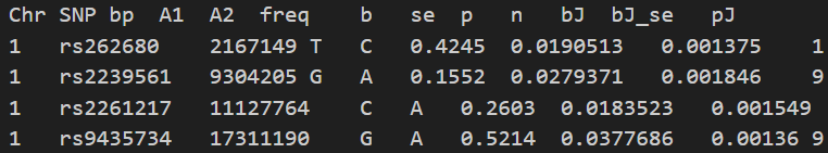
In the output file, each row corresponds to a single SNP:
Chr SNP bp A1 A2denote the chromosome, SNP ID, base-pair position, the effect allele, and the other allele specified in the.bimfile.freq b se pare taken from the input GWAS summary statistics file.nis the estimated effective sample size for analysis (different fromNin GWAS summary statistics).bJ bJ_se pJrepresent the joint effect size, standard error, and p-value from a joint analysis of all the selected SNPs.
You can verify that your output file is identical to the provided example output file by running diff Height_analysis.jma.cojo Height_analysis.jma.cojo.example. If the command produces no output, this confirms that the software is running correctly on your machine.
People are often interested in these three columns SNP, A1, and bJ, which can be directly used to compute polygenic scores with the PLINK –score function. SNP, A1, and bJ correspond to [variant ID col.], [allele col.], and [score col.], respectively.
Step 3: Run conditional or joint analysis
In some cases, users may wish to perform conditional analysis or joint analysis separately. This requires providing a list of SNPs of interest. As an example, we use the SNPs selected in the previous step.
Run the following command to perform joint analysis:
./manc_cojo \
--bfile 1KGPhase3.w_hm3 \
--cojo-file Height.sumstat \
--out Height_analysis_joint \
--extract Height_analysis.jma.cojo 2 header \
--cojo-joint
--extract Height_analysis.jma.cojo 2 header indicates that only SNPs listed in the file Height_analysis.jma.cojo are included in the analysis, SNP IDs are read from the second column of the file, and the file contains a header line.
Because the joint effects are computed using the same input files and the same set of selected SNPs, the output file Height_analysis_joint.jma.cojo should be identical to Height_analysis.jma.cojo generated in Step 2.
Run the following command to perform conditional analysis:
./manc_cojo \
--bfile 1KGPhase3.w_hm3 \
--cojo-file Height.sumstat \
--out Height_analysis_cond \
--cojo-cond Height_analysis.jma.cojo 2 header
This will produce an output file named Height_analysis_cond.cma.cojo. Note that .cma.cojo files are often very large.
Step 4: Extend to multi-ancestry analysis
To extend the analysis to multiple ancestries, simply provide multiple GWAS summary statistics and LD reference panels.
As a minimal example, suppose we have two cohorts with identical input files. Multiple cohorts are specified by appending additional file paths after --bfile and --cojo-file:
./manc_cojo \
--bfile 1KGPhase3.w_hm3 1KGPhase3.w_hm3 \
--cojo-file Height.sumstat Height.sumstat \
--out Height_analysis_two_cohorts \
--cojo-slct
In the output file, you will now see a header like:
Chr SNP bp A1 A2 freq.1 b.1 se.1 p.1 n.1 bJ.1 bJ_se.1 pJ.1 freq.2 b.2 se.2 p.2 n.2 bJ.2 bJ_se.2 pJ.2 bJ.ma bJ_se.ma pJ.ma
Chr SNP bp A1 A2have the same meanings as described above, whereA1andA2are unified according to the.bimfile of cohort 1.freq.1 b.1 se.1 p.1 n.1 bJ.1 bJ_se.1 pJ.1, andfreq.2 b.2 se.2 p.2 n.2 bJ.2 bJ_se.2 pJ.2have the same meanings as described above, with the suffixes.1and.2indicating the cohort index (i.e., cohort 1 and cohort 2).bJ.ma bJ_se.ma pJ.mareport the joint effect size, standard error, and p-value from multi-cohort joint analysis of all selected SNPs across both cohorts.
-
Publicly available from 1000 Genomes. We use PLINK to merge the 22 chromosomes into a single bfile for convenience. ↩